For the basic equations of fluid mechanics (Navier-Stokes equations or mass, – momentum and energy conservation equations) no analytical solutions are known, except for special cases like the plane plate. An analytical solution would be, for example, an equation for the density ρ as a function of the other quantities u, v, w, e.
Therefore, the differential equation system must be solved numerically for technically relevant problems. For this purpose, the partial derivatives (differentials) must be converted into finite differences. This is called discretization. The discretized differential equations are then called difference equations. These difference equations can be solved on a so-called computational mesh. In the numerical solution, the numerical values for the flow variables are then available as ρ, u, v, w, e at the mesh points.
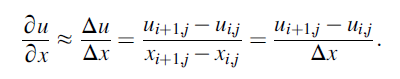
Figure below shows a small section of a two-dimensional computational mesh with nine mesh points. The solution is calculated only at these grid points. A so-called cell corner point scheme is shown here, where the grid points are located on the corners of the volume element. Alternatively, they can also be located inside the volume element. The volume element is then offset by half a mesh size and is referred to as a cell center method. Discretization thus means that in the differential equations the differentials are replaced by differences. For example, the differential of the velocity in ∂u/∂x x-direction at the point
can be P(i, j) replaced by the difference of the values at the neighboring points and (i + 1, j) (i, j)
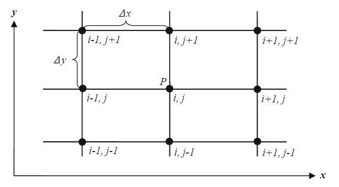
Schematic of a computational mesh around the point P
Three methods of discretization are distinguished, but they are equivalent and can be transferred into each other: the finite difference, the finite volume and the finite element discretization. Each method has its advantages and disadvantages:
- The finite difference (FD) discretization is very illustrative and is used below to show the principle of discretization. It uses the conservation equations in differential form (Chap. 2). The grid points are located at the corners of the volume element (cell corner point scheme).
- Finite volume (FV) discretization is very accurate for discontinuities such as shocks, which is why modern CFD programs mostly use this method. It uses the conservation equations in integral form and the integrals are replaced by sums. The support points are either located inside the volume element (cell center scheme) or, as in the FD discretization, at the corners (cell corner point scheme).
- The finite element (FE) method is preferred by mathematicians because it is mathematically easy to represent. In this method, mathematical equations such as straight line or parabolic equations are used for the differentials.
Figure below shows that finite difference (FD) methods have the highest accuracy and finite element (FE) methods have the highest flexibility. In practice, the finite volume (FV) methods have prevailed in the commercial CFD programs, since they have a good accuracy and flexibility.
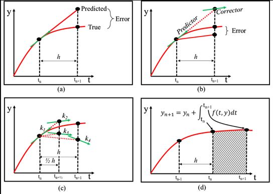
Since the discretization methods are different, a distinction is made between the discretization of the spatial derivatives and the temporal derivative.
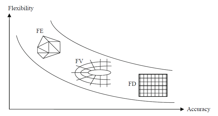
Classification of discretization methods. (According to Laurien and Oertel)
Source : Computational Fluid Dynamics : Getting Started Quickly With ANSYS CFX 18 Through Simple Examples by Stefan Lecheler