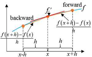
The Finite Difference Method (FDM) is an Eulerian method that involves approximating the derivative of a function using finite differences. It relies on a previously defined spatial discrete mesh of nodes. The starting point is the Newton-Raphson method, where the derivative of the function at a point equals the slope of the tangent line to the function (curve) at that point.
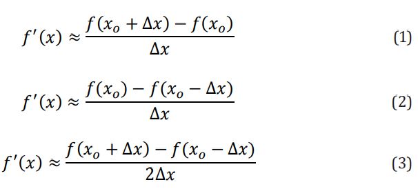
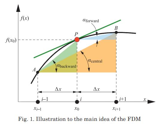
This concept is illustrated in Figure 1. However, this definition is not unambiguous because it can be implemented in at least three ways: the so-called forward scheme (1), the backward scheme (2), or the central scheme (3)
In equations (1-3), only three nodes are utilized (i – 1, i, i + 1). However, higher order numerical schemes can also be structured, involving 5 or more nodes to approximate a derivative. The second derivative of the function f(x) at the point x0 is obtained by applying the difference scheme three times. Depending on the schemes employed, there can be multiple variations of the second derivative.
It should be noted that if the equation includes a time-dependent term, time must also be discretized. The maximum allowable time step depends on the numerical scheme utilized and is sometimes constrained by additional parameters, primarily the CFL condition.
The idea of the finite difference method is to use the above quotient,
, to approach the gradient (derivative) at the point , point or any point between them. The geometric analogy of this approximation is to use a secant line to approximate a tangent line. For the first-order derivative, the most common schemes are forward, backward, and central difference schemes. A forward scheme has an expression of the formIt is called “forward” because we use the function value at a point in front of (along the direction of the corresponding axis) the point at which the derivative is calculated. Likewise, a backward scheme uses the function values at and instead:We can also approximate the derivative using the function values at points on the two sides of the point of derivative asA second-order derivative can be approximated using first order derivatives as we can view the second-order derivative as a derivative of first-order derivatives. For example, in order to obtain the second-order derivative at the point , we can use the derivatives at the points and :The above approximation uses the central difference. We can also use central differences for the first derivative in the above equation, leading to
Temporal Finite Difference and Schemes
Let us first reformulate the general transient partial differential equation in the following way:where in the equation contains all the terms except the temporal derivative term. First, for the temporal difference, let us use the following most common form as our purpose is to calculate the function value at the next time step based on the known function value at the current time step :where is the time step. An Euler forward scheme is used for the temporal derivative. The word “Euler” differentiates the temporal schemes from the spatial schemes. The choice of , i.e. from which time step, determines the type of the temporal scheme. If all the unknown values are from the current step, then the scheme is explicit,The following solution can be readily obtained for this scheme:The above two types of schemes can also be mixed to construct other schemes:where is the ratio. values of 0 and 1 lead to explicit and fully implicit schemes, respectively; while those values between 0 and 1 produce partially implicit ones. Another common implicit scheme, the Newton-Nicolson scheme will be obtained when equals 0.5. Partially implicit schemes are also unconditionally stable.
Example
Let us consider the following problem, where,Let us discretize the domain with a length of into points, for which we have . The physical process to be simulated lasts a time period of . Then the discretization starts with the temporal and spatial discretization at each point:Point 1: Point 2: Point : Point : If we incorporate the above boundary conditions, we will getPoint 1: Point 2: Point : Point :
The above series of equations can be represented using the following algebraic equation:The initial condition is applied in the first step of the iteration when The discretized function value for the first step is